This section describes our progressive
design method to minimize the effects of large search spaces and the
bootstrap problem when evolving a controller for a robot whose
morphology, task and environment are fixed and complex. It is based on
staged evolution, and extends it by providing a standard building block
and evolutionary method for any robot, independent of its number of
sensors or actuators. In the progressive design method, architectural
modularity is created at the robot device level by creating a small and
independent neural module around each of the robot’s sensors and
actuators. This change in modularity has in chapter 5 been proven to be
more effective than other modularization approaches, and it
additionally adds the advantage of allowing a very flexible learning
modularization.
Basically, the progressive design
process works as follows: at the beginning of the evolutionary process
a limited number of modules are evolved in a bounded evaluation task.
Following this the rest of the modules are added in successive stages,
with only the newly added modules and their connections with the
already evolved ones in previous stages being evolved. The final global
controller is then gradually evolved in a process referred to as
progressive design of complex neural controllers.
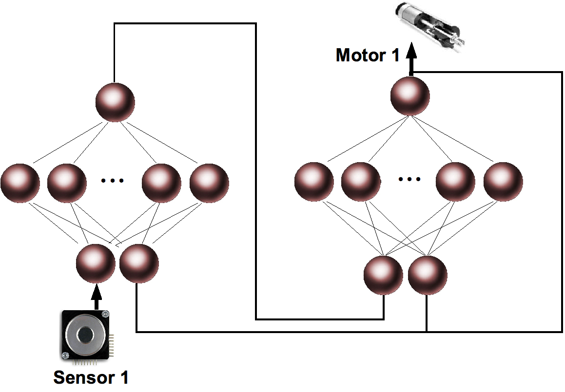
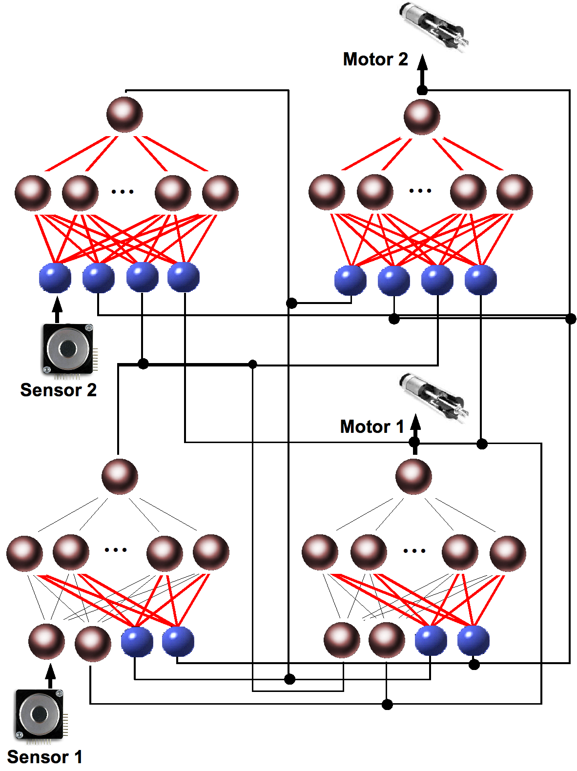
Figure 6.1: The first example of the progressive design of a neural
controller for
a simple robot with two sensors and two actuators. In stage one (top),
only one
IHU for sensor 1, and one IHU for motor 1 are evolved, using a given
fitness
function f1, and obtaining the controller on the top. In stage two
(bottom), two
additional IHU’s (for sensor 2 and motor 2) are added to the
controller. At this
stage, only those newly added modules and their connections to the
previously
evolved modules (red lines) are evolved by using a different fitness
function f2.
Bias information is used to decide which IHU’s are going to be evolved
first,
with which combination and using which fitness function. Hence, the
designer
requires knowledge of the domain.
This section shows results obtained
when the methodology is applied to the Aibo robot for the generation of
a walking behaviour. The generation of such a behaviour is a complex
issue, since Aibo endows 12 DOF’s related to walking, with no head or
queue DOF being taken into account. Each leg has 3 DOF’s that must be
coordinated between all the legs. It is easy to see that a
miscoordination in one single joint may cause the robot to fall.
For the generation of the walking gait
only the motors in the leg joints and those corresponding joints
sensors will be taken into account. Neither the paw sensors nor the
accelerometers will be used in this case.
The whole process will be carried out
in simulation, and once finished it will be transferred to the real
robot and tested on it.
A CTRNN will be used in each IHU processing element. The CTRNNs will
implement an oscillatory behavior (a CPG) for each joint of the robot.
The method will then evolve in stages the oscillatory patterns of each
joint and at the same time, generate a coordination between the
oscillators that allows the robot to walk.
The walking behavior required to perform the evolution in three stages:
First the CPGs are evolved
Then
CPGs of a same type are interconnected, evolving the coordination
weights. This leads to the obtention of three different layers of CPGs
Last, the three layers are interconnected and the coordination
weights evolved.
First stage: generation of the joint oscillator
The aim of this stage is to obtain a controller for a joint by
generating an oscillatory pattern for each type of robot joint. Joints
in the robot’s legs are of three different types, which we will call
J1, J2 and J3. J1 is in charge of the rotatory movement of the
shoulder, J2 of the lateral movement of the shoulder and J3 of the knee
movement.
The DAIR architecture described in chapter 4 is applied to a single
joint composed of two devices. An oscillator is implemented for each
joint by coupling two IHU (one for the joint sensor and another
for the motor), each one having a CTRNN networks. Both nets
are interconnected as specified by the architecture, but each one is in
charge of a different element: the sensor net is in charge of the
sensor, and the motor net in charge of the motor.
The fitness function used for the evolutionary process is:
fitness = fit_var ∗ fit_cross
where fit_var is the variance of the joint position during the 200
evaluation steps, and fit_cross is the number of times that the joint
crosses in its movement through the mean positional value.
The oscillation obtained for J1 can be observed in the following video:
Second stage: generation of two coupled oscillators
The aim of the second stage is to obtain a controller for two joints of
the same type, in a coupled oscillation within a given phase
relationship. In this case, the controller will now be composed of four
neural networks (for each type of joint): two controlling the two
motors and two controlling the two sensors.
A duplication of the modules created in the previous stage will be
performed for the new joint and just the connections between modules
will be evolved. The oscillator controlling one type of joint from the
previous stage will be copied to control the joint of the same type,
i.e. the joint that is opposite the original one, thereby obtaining two
isolated oscillators. Connections between both modules are then
established in order to apply the architecture definition, and only
these connections need to be evolved in this stage. A phase relation of
PI rad between those two legs (in all types of joints) will be required.
The fitness function used is the following
fitness = fit_cross1 ∗ fit_cross2 ∗
fit_var
where fit_var is the variance for the difference of positions between
both legs
during the 400 evaluation steps, and fit_cross1 and fit_cross2 are the
number
of crossings that each joint has performed through its mean position
value.
The resulting oscillation for joint type J1 can be seen in the
following video:
Third stage: coupling the oscillation of four joints of the same
type
In this stage, the control for the rear two joints of the same type is
added to the controller. This means that four new neural modules will
be added to the modular controller: two for the control of the two rear
joints, and two for the two rear sensors. However, since the two front
joints have the same phase relationship for a walking gait as the two
rear joints have, it is possible to clone the controller obtained for
the front joints for the rear joints, and then evolve only the
connections between them.
the following
The fitness function:
fitness = fit_cross ∗ fit_oscil ∗
fit_phases
where fit_cross is the product of the number of crossings for each
joint performed through their mean positional value, fit_oscil is the
variance of the left fore joint which indicates how well that joint
oscillates, assuming that if this joint oscillates the others must
follow, and fit_phases is the part of the fitness that indicates the
phase relationship between all the joints.
The resulting oscillation can be observed in the following video:
Fourth stage: coupling between types of joints
The last stage is the coupling between the three groups of neural
controllers obtained. What is now required is to connect the three
layers in order to obtain a coordination between the different joint
types to enable the robot to walk, and to complete the architecture as
a whole.
A new fitness function was proposed where the oscillation of the joints
was still imposed, together with the distance walked. If the robot does
not fall over the fitness function is composed of two multiplying
factors: the distance d walked by the robot in a straight line and the
phase relationship between the different joints. If the robot does fall
over the fitness is zero.
Using
the proposed method we achieved a quick and dynamic gait for Aibo. You
can check yourself the results by looking at the following videos or
trying the code below
Real robot controller used:
You can test our results on your own Aibo robot, by downloading from
here the OPEN-R neural controller and the neural nets evolved. Just
download the OPEN-R program, unpack it and install it in the /MS/OPENR
directory of an already prepared OPEN-R memory stick (if you don't know
how to do it, please read the 'Aibo Quickstart
Manual'). Then download the neural nets, unpack them and install
them into the /MS/OPENR/MW/DATA/P directory of your memory
stick.
By running the program on Aibo, the robot will perform a series of
walking steps, governed by the neural nets, and then it will stop for
some seconds for recording the joints stored values in memory (MS
writting is very slow). A file called MSV.csv will be created
in the /MS/OPENR/MW/DATA/P
directory containing all the joint positions recorded during walking.
After it has been written, the robot will continue walking again for
some other steps.
The real robot results presented above run onboard the robot by
using the cross-compilation feature of Webots. However, it is possible
to use the URBI programming
interface to run the neural controller in C++ on a computer,
controlling the real robot wirelessly from the computer. This is
possible using libUrbi in two different modes, synchronous and
asynchronous. Our tests show that synchronous mode is not suitable for
this highly dynamic task and that asynchronous mode is more appropriate
and close to the onboard control.
libURBI robot controllers used:
In order to test our results on your own Aibo robot, you need to
download and install first the URBI server on a memory stick, and the
libURBI libraries on your computer. Then compile and execute the code
provided below. Libraries required for the linkage between libUrbi and
the neural net functions are provided within the same files.
Web page by R. Téllez using rubric css by Hadley
Wickham
Don't undertake a project unless it is
manifestly important and nearly impossible (Edwin Land)